From Spectrum to Foster Network
Once the logarithmic time-constant spectrum \(R(\zeta)\) is known (via Fourier, Bayesian or LASSO deconvolution) the first physical network we construct is the Foster ladder.
Discrete Foster elements
Discretise the spectrum into bins of width \(\Delta\zeta_i\) centred at \(\zeta_i=\ln\tau_i\) (see From spectrum to RC network). For each bin
exactly the formulas used in network identification by deconvolution. Every tuple \((R_i,C_i)\) corresponds to one parallel RC branch whose time-constant is \(\tau_i=R_iC_i\).
Piece-wise construction of the impedance
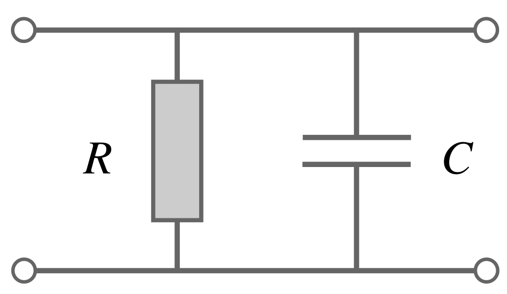
Fig. 4 Parallel RC element |

Fig. 5 Two parallel RC elements connected in series |
A single parallel RC branch driven in series has
Because the branches are stacked in series, the input impedance of the Foster ladder is the sum of the individual impedances:
Equation (54) is simply the partial-fraction form produced by the pole–zero representation (§“Lumped element RC lines”). Building \(Z(s)\) “piece by piece” is therefore trivial:
start with \(Z^{(1)}(s)=Z_1(s)\);
for k = 2 … n: \(Z^{(k)}(s)=Z^{(k-1)}(s)+Z_k(s)\).
Pole–zero representation
After summing the parallel branches (Equation (54)) the overall impedance can also be written in pole–zero form
Poles Each Foster branch contributes a real pole
(56)\[\sigma_{p,i}=\frac{1}{\tau_i} =\frac{1}{R_iC_i},\]located on the negative real axis.
Zeros The finite zeros \(\sigma_{z,k}\) fall between adjacent poles; they arise automatically from the summation of terms in Equation (54). Pole–zero interlacing guarantees that \(Z(s)\) is a positive-real function, hence physically admissible for a passive one-port.
Low- and high-frequency limits
(57)\[Z(0)=R_{\infty}, \qquad Z(\infty)=0,\]matching the expected behaviour of a purely diffusive thermal path.
The pole–zero picture provides an immediate diagnostic: widely separated poles imply well-resolved thermal layers, while closely spaced poles hint at a continuous-diffusion region that may be better represented by a non-uniform RC line.